2024-06-1617:39 Status:Complete
Fundamental SI and Derived Units
Derived units are combinations of fundamental units. Some examples are:
- m/s (Unit for velocity)
- N (kg*m/s^ (Unit for force)
- J (kgm^2/s^2) (Unit for energy) However the fundamental units are as follows:
| Quantity | SI unit | Symbol |
|---|---|---|
| Mass | Kilogram | kg |
| Distance | Meter | m |
| Time | Second | s |
| Electric current | Ampere | A |
| Amount of substance | Mole | mol |
| Temperature | Kelvin | K |
Scientific Notation and Metric Multipliers
In scientific notation, values are written in the form , where is a number between 1 and 10 and is any integer. Some examples are:
- The speed of light is . In scientific notation, this is expressed as
- A centimeter (cm) is 1/100 of a meter (m). In scientific notation, one cm is expressed as .
| Prefix | Abbreviation | Value |
|---|---|---|
| peta | P | 10^15 |
| tera | T | 10^12 |
| giga | G | 10^9 |
| mega | M | 10^6 |
| kilo | k | 10^3 |
| hecto | h | 10^2 |
| deca | da | 10^1 |
| deci | d | 10^-1 |
| centi | c | 10^-2 |
| milli | m | 10^-3 |
| micro | μ | 10^-6 |
| nano | n | 10^-9 |
| pico | p | 10^-12 |
| femto | f | 10^-15 |
Significant Figures
For a certain value, all figures are significant, except:
- Leading zeros
- Trailing zeros if this value does not have a decimal point, for example:
- 12300 has 3 significant figures. The two trailing zeros are not significant.
- 012300 has 5 significant figures. The two leading zeros are not significant. The two trailing zeros are significant.
When multiplying or dividing numbers, the number of significant figures of the result value should not exceed the least precise value of the calculation.
The number of significant figures in any answer should be consistent with the number of significant figures of the given data in the question.
Orders of Magnitude
Orders of magnitude are given in powers of 10, likewise those given in the scientific notation section previously.
Orders of magnitude are used to compare the size of physical data.
| Distance | Magnitude (m) | Order of magnitude |
|---|---|---|
| Diameter of the observable universe | 10^26 | 26 |
| Diameter of the Milky Way galaxy | 10^21 | 21 |
| Diameter of the Solar System | 10^13 | 13 |
| Distance to the Sun | 10^11 | 11 |
| Radius of the Earth | 10^7 | 7 |
| Diameter of a hydrogen atom | 10^-10 | 10 |
| Diameter of a nucleus | 10^-15 | 15 |
| Diameter of a proton | 10^-15 | 15 |
| Mass | Magnitude (kg) | Order of magnitude |
| The universe | 10^53 | 53 |
| The Milky Way galaxy | 10^41 | 41 |
| The Sun | 10^30 | 30 |
| The Earth | 10^24 | 24 |
| A hydrogen atom | 10^-27 | -27 |
| An electron | 10^-30 | -30 |
| Time | Magnitude (s) | Order of magnitude |
|---|---|---|
| Age of the universe | 10^17 | 17 |
| One year | 10^7 | 7 |
| One day | 10^5 | 5 |
| An hour | 10^3 | 3 |
| Period of heartheart | 10^0 | 0 |
Random and Systematic Errors
| Random error | Systematic error |
|---|---|
| - Caused by fluctuations in measurements centered around the true value (spread). - Can be reduced by averaging over repeated measurements. -Not caused by bias. | - Cannot be reduced by averaging over repeated measurements. - Caused by fixed shifts in measurements away from the true value. - Caused by bias. |
| Examples: - Fluctuations in room temperature - The noise in circuits - Human error | Examples: - Equipment calibration error such as the zero offset error - Incorrect method of measurement |

Absolute, Fractional and Percentage Uncertainties
Physical measurements are sometimes expressed in the form x±Δx. For example, 10±1 would mean a range from 9 to 11 for the measurement.
| Absolute uncertainty | Δx |
|---|---|
| Fractional uncertainty | Δx /x |
| Percentage uncertainty | Δx/x*100% |
| Calculating with uncertainties |
| Addition/Subtraction | y=a±b | Δy=Δa+Δb (sum of absolute uncertainties) |
|---|---|---|
| Multiplication/Division | y=a*b or y=a/b | Δy/y=Δa/a+Δb/b (sum of fractional uncertainties) |
| Power | y=a^n | Δy/y= |
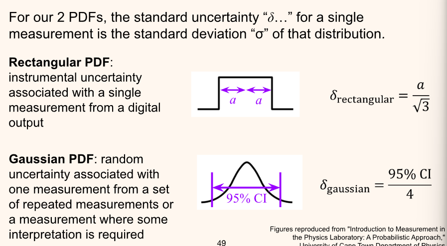
Instrumental (Rectangular) Uncertainties
Keep in mind that there is always a combination of both Gaussian and Instrumental uncertainty. Use the appropriate one depending on which one dominates. For instance when stopping a stopwatch the error comes primarily from the time needed for a person to register the measurement and mechanically record it. There is some instrumental uncertainty (even if the press was precise), however, the Gaussian error made from the delay in stopping the stopwatch would dominate the rectangular error of the instrument.
Instrumental Uncertainty
Take a balance of some chemical powder in a scale, dependent on the calibrated masses. Consider that even the smallest difference of mass will cause the arms to swing to the other side.
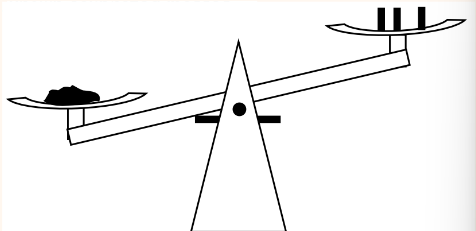
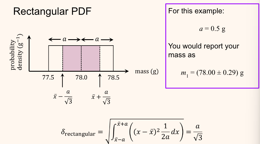
For this reason, a rectangular probability density is used to describe uncertainty (As opposed to Gaussian). Similar to a digital reading of “0.78”, it is unknown how likely the value displayed is the actual value. For this reason, when using an instrument, read the displayed/specified/implied (e.g. if a scale has a precision of 0.01, the uncertainty is 0.005…) uncertainty on the instrument.
To find the confidence interval of a rectangular distribution perform the following as done in this example:
Gaussian Uncertainties
For “random error” or other error produced by human fault. To visualize this, take measurements and plot them on a curve. If they look similar to a Gaussian curve (normal distribution), then the dominant error is from “random error.”
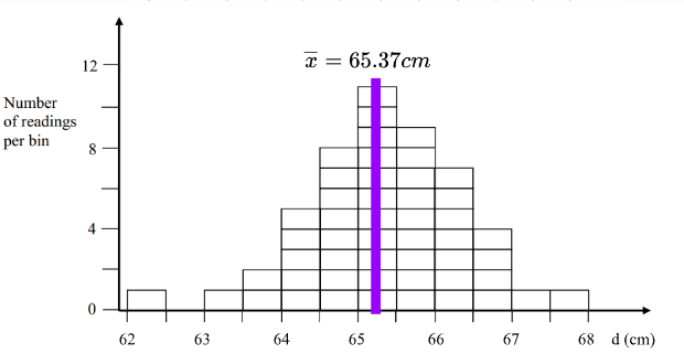 Where is the number of times the measurement is taken, and is the value of the measurement. These can be used to find the standard deviation (describing how narrow/wide the distribution is).
Where is the standard deviation. is used to find how far the data point at is. It is the square to make it positive (later undone by the square root). The sum of all the distances from the mean, is then divided by the trials, (excluding itself ).
Where is the number of times the measurement is taken, and is the value of the measurement. These can be used to find the standard deviation (describing how narrow/wide the distribution is).
Where is the standard deviation. is used to find how far the data point at is. It is the square to make it positive (later undone by the square root). The sum of all the distances from the mean, is then divided by the trials, (excluding itself ).
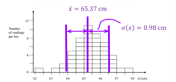
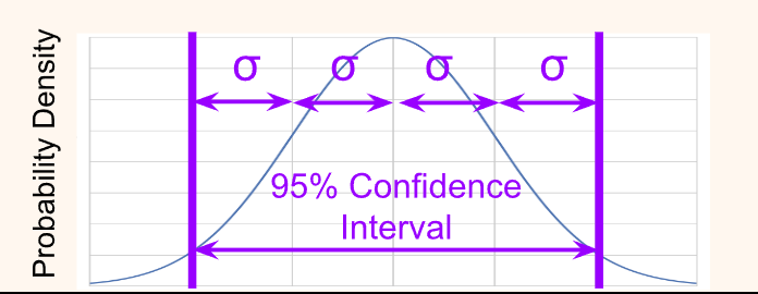
To simplify calculations, a confidence interval (CI) is taken at
Summary
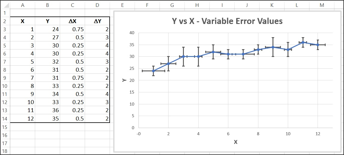
Error Bars
Data represented that have error bars are bars on graphs which indicate uncertainties. They can be horizontal or vertical, with the total length of two absolute uncertainties.
Correlation
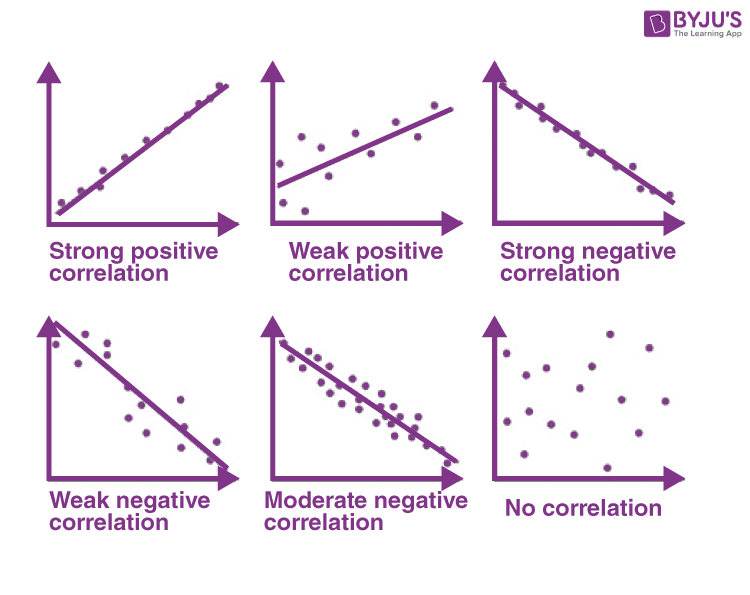
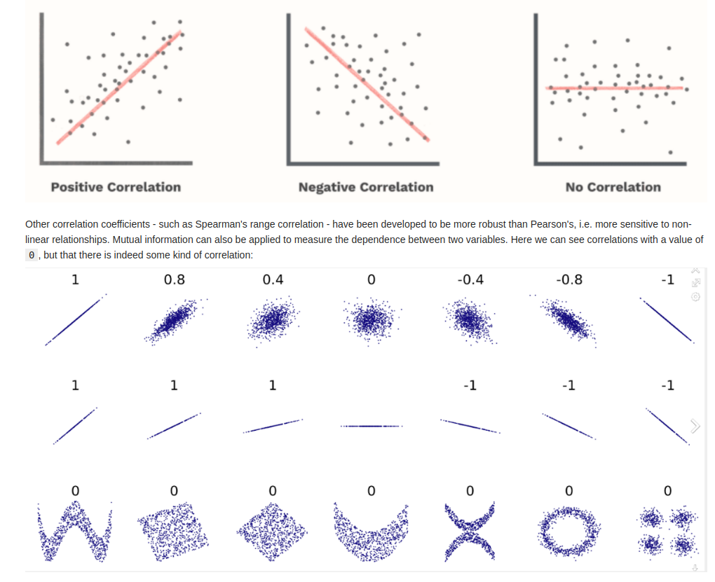
- NOTE: a strong linear correlation with a slope or r = 0 is still considered to have no correlation.